Exercise 1. Import Census and Municipal Geometries

Population Profiling with R, August 2024

1 Summary

In this exercise, we will import and map the following datasets for Camden County, NJ:

• county boundary
• census tracts (2020)
• census blocks (2020)
• zip code tabulation areas (ZCTAs) (2020)
• municipalities
• wards

As we import them, we will:

• make sure they are in the same CRS (specifically geographic coordinates NAD83, EPSG:4269)
  
• save copies to disk so we can use them in other notebooks

This notebook will feature functions from the following packages:

• tigris
• sf
• dplyr
• arcgislayers
• ggplot

2 Spatial Data from the US Census Bureau

The US Census Bureau is a good choice for spatial data for the following reasons:

• they are an official government source
• they provide boundaries for a wide range of spatial units researchers like to work with, from States all the way down to Census Blocks (see diagram below)
• they also publish other kinds of spatial units, including things like zip codes, school districts and congressional districts (complete list)
• you can import boundaries via an API (i.e., don’t have to go to a website and download zip files)
• they come with a standard identifier (i.e., geoid) that the Census Bureau and many other data publishers use when publishing socio demographic data
• they provide historical data for statistical areas that change over time (e.g., census enumeration units)
• the tigris and tidyCensus packages make downloading them easy

2.1 Setup

First we load the packages we’ll be needing:

library(dplyr)
library(ggplot2)
library(sf)

The main package we’ll be using to download spatial data from the US Census is tigris. You do not need an API key to download spatial data from the Census.

library(tigris)

To enable caching of data, set `options(tigris_use_cache = TRUE)`
in your R script or .Rprofile.

tigris supports caching for the files it downloads, which we certainly want to enable:

options(tigris_use_cache = TRUE)

2.2 Set Up a Local Data Directory

We also want to save the spatial files we download to our hard drive, so we can use them in other notebooks.

We’ll do this by creating a folder in your operating system’s ‘AppData’ folder, and copies of our “finished products” there.

my_data_dir <- tools::R_user_dir("datafordemocracy", which = "data")
if (!dir.exists(my_data_dir)) dir.create(my_data_dir, recursive = TRUE)
tools::file_path_as_absolute(my_data_dir)

[1] "C:/Users/Andy/AppData/Roaming/R/data/R/datafordemocracy"

2.3 Import the County Boundary

The tigris package doesn’t have a function to download a single county boundary. So we start by getting all the counties in NJ:

nj_counties_sf <- tigris::counties(state = "NJ", cb = TRUE, progress_bar = FALSE)

Retrieving data for the year 2022

nj_counties_sf |> head()

Notes

• GEOID is the unique identifier for each county. It is a combination of STATEFP (State ID) and COUNTYFP (county number within the state).
  
• the CRS is geographic coordinates in NAD83 (EPSG:4269)
  
• cb = TRUE tell it to return a ‘cartographic boundary’ file (i.e., with water bodies removed)

Pull out just Camden county:

camden_bnd_sf <- nj_counties_sf |> filter(NAME == "Camden")

Plot it:

ggplot(camden_bnd_sf) + 
  geom_sf() + 
  labs(title = "Camden County, NJ")

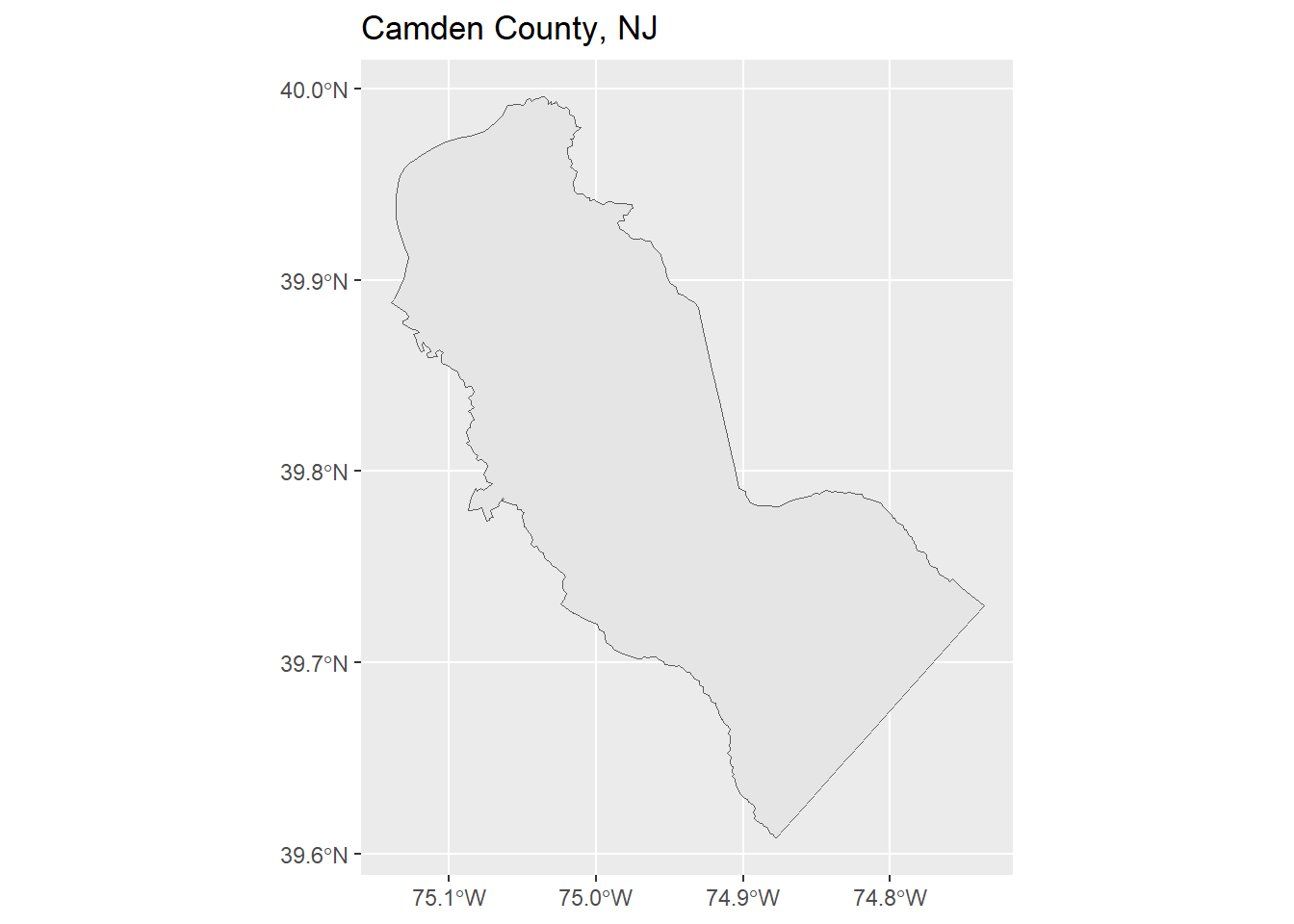
Save a copy to disk:

saveRDS(camden_bnd_sf, file.path(my_data_dir, "camden_bnd_sf.Rds"))

2.4 CHALLENGE

Import and plot the county boundary where you live or work.

## Your answer here

2.5 Import Census Tracts

Census tracts are designed to have about ~4,000 people. They are not the smallest unit, but they are important enumeration units because many of the census variables are only available at the tract level and larger.

camden_tracts20_sf <- tigris::tracts(state = "NJ", county = "Camden", year = 2020, 
                                     cb = TRUE, progress_bar = FALSE)
nrow(camden_tracts20_sf)

[1] 129

head(camden_tracts20_sf)

Note: The GEOID values are 10-digits wide (combination of state, county, and tract ID values).

Map the census tracts

Next, we plot the census tracks and the county boundary together.

Check the CRS Before Plotting

ggplot() does not do projection on-the-fly, so before we overlay the census tracts and county boundary, we need to verify they are in the same CRS:

identical(st_crs(camden_tracts20_sf), st_crs(camden_bnd_sf))

[1] TRUE

ggplot(camden_tracts20_sf) + 
  geom_sf() + 
  geom_sf(data = camden_bnd_sf, fill = NA, lwd = 1.2) +
  labs(title = "Camden County Census Tracts",
       subtitle = "2020 Census")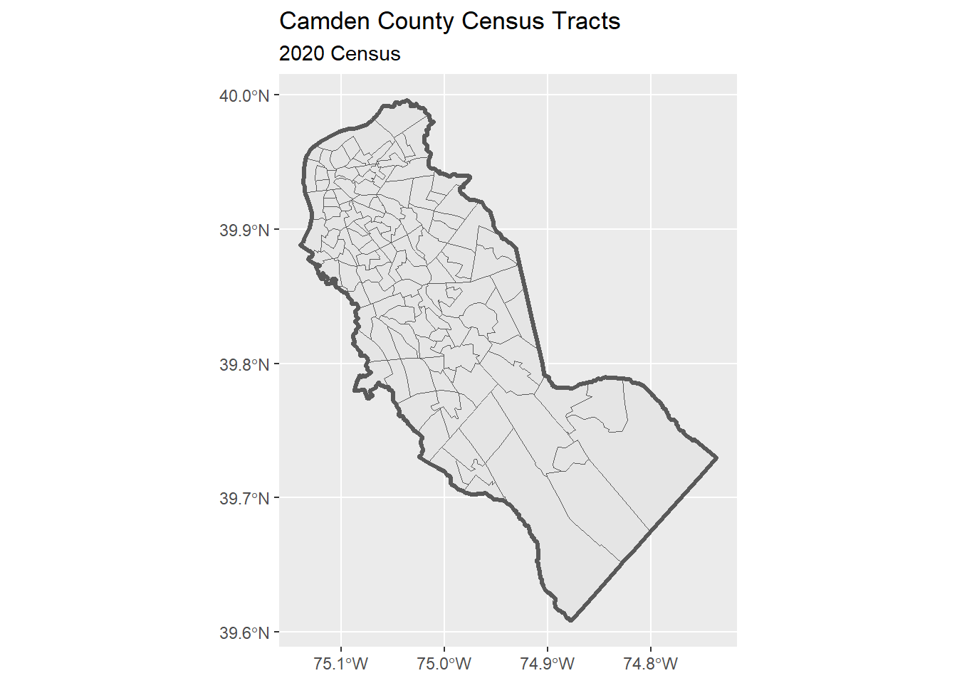

Save a copy:

saveRDS(camden_tracts20_sf, file.path(my_data_dir, "camden_tracts20_sf.Rds"))

2.6 Import Census Blocks

Using a similar approach as above:

camden_blks20_sf <- tigris::blocks(state = "NJ", county = "Camden", year = 2020, progress_bar = FALSE)
nrow(camden_blks20_sf)

[1] 8770

Plot:

ggplot(camden_blks20_sf) + 
  geom_sf() + 
  geom_sf(data = camden_bnd_sf, fill = NA, lwd = 1.2) +
  labs(title = "Camden County Census Blocks, NJ",
       subtitle = "2020") +
  theme_light()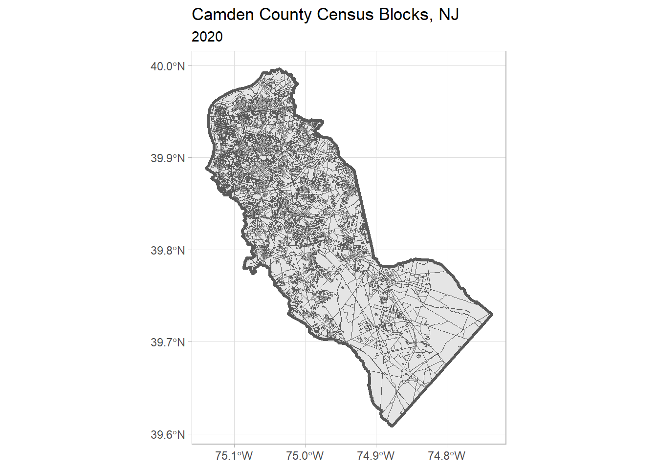

Save a copy:

saveRDS(camden_blks20_sf, file.path(my_data_dir, "camden_blks20_sf.Rds"))

2.7 CHALLENGE

Import and plot the block groups for YOUR county.

## Your answer here

2.8 Import Zip Codes

Zip codes are not ideal for spatial analysis, but sometimes that’s all the location reference we have.

We can import Zip Code Tabulation Areas (zctas), which are roughly the boundaries of zip codes (details).

ztacs don’t have the name of a county as an attribute, so we have to take a different approach to select the ones we want to keep.

Import zcta’s that start with 08 (southern half of New Jersey):

## Uncomment the following to download the ZCTAs from the census API
## zcta_08_sf <- tigris::zctas(year = 2020, starts_with = "08", progress_bar = FALSE)

## Load a saved copy
zcta_08_sf <- readRDS(here::here("exercises/data/zcta_08_sf.Rds"))

nrow(zcta_08_sf)

[1] 290

head(zcta_08_sf)

Plot them:

ggplot(zcta_08_sf) + 
  geom_sf() + 
  geom_sf(data = camden_bnd_sf, fill = NA, col = "red", lwd = 1.1) +
  labs(title = "Zip Code Tabulation Areas that Start with 081",
       subtitle = "2020")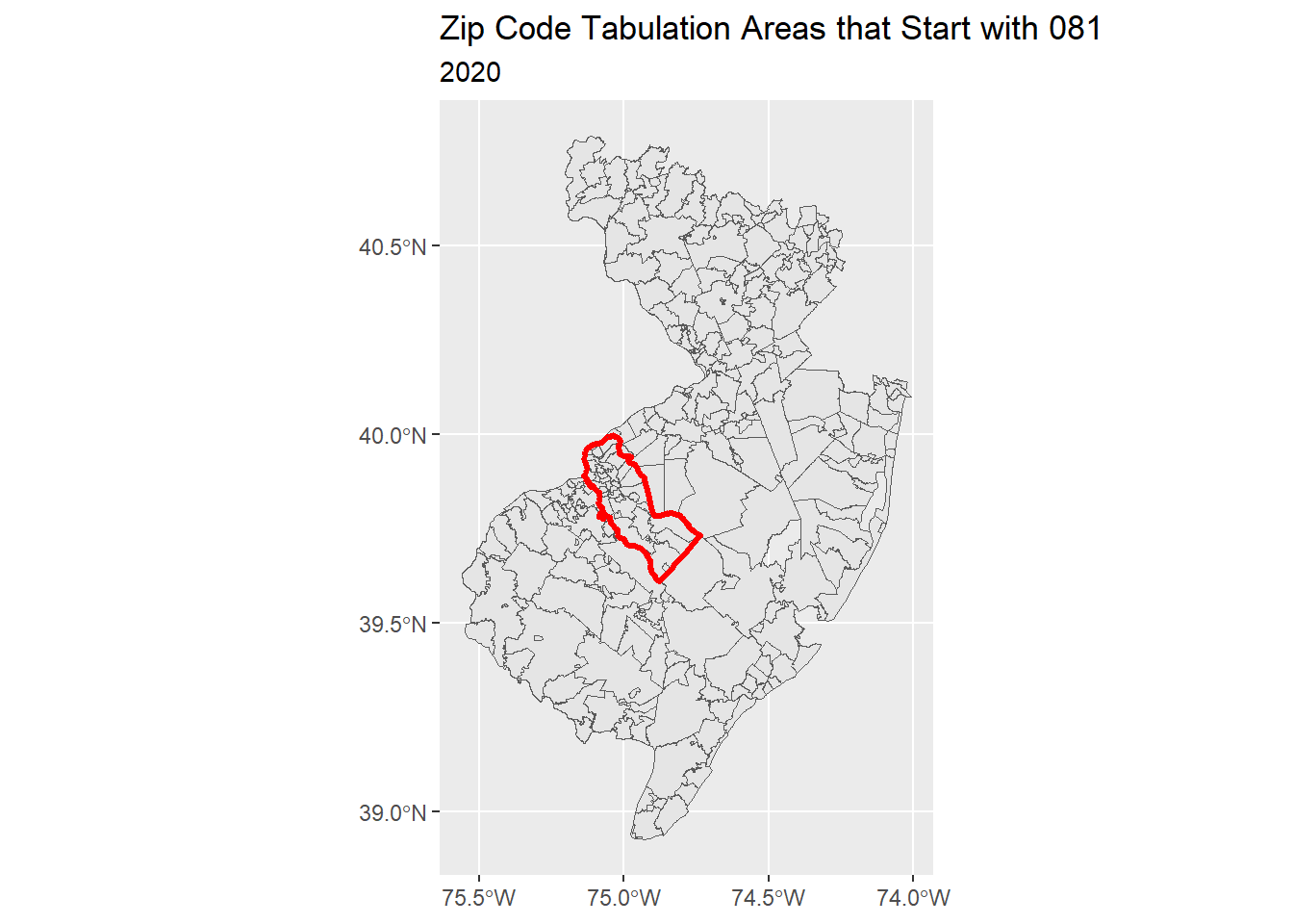

To select the zctas we want to keep, we have to do a spatial query:

camden_zcta20_sf <- zcta_08_sf |> 
  st_intersection(camden_bnd_sf)

Warning: attribute variables are assumed to be spatially constant throughout
all geometries

nrow(camden_zcta20_sf)

[1] 47

Plot the Camden ZCTAs:

## Define a color pallete
rand_cols <- nrow(camden_zcta20_sf) |> 
  rainbow(end=5/6) |> 
  sample(size = nrow(camden_zcta20_sf), replace = TRUE)

ggplot(camden_zcta20_sf) + 
  geom_sf(fill = rand_cols, alpha = 0.3) + 
  geom_sf(data = camden_bnd_sf, fill = NA, lwd = 1.2) +
  labs(title = "Camden County 081 ZCTAs, NJ")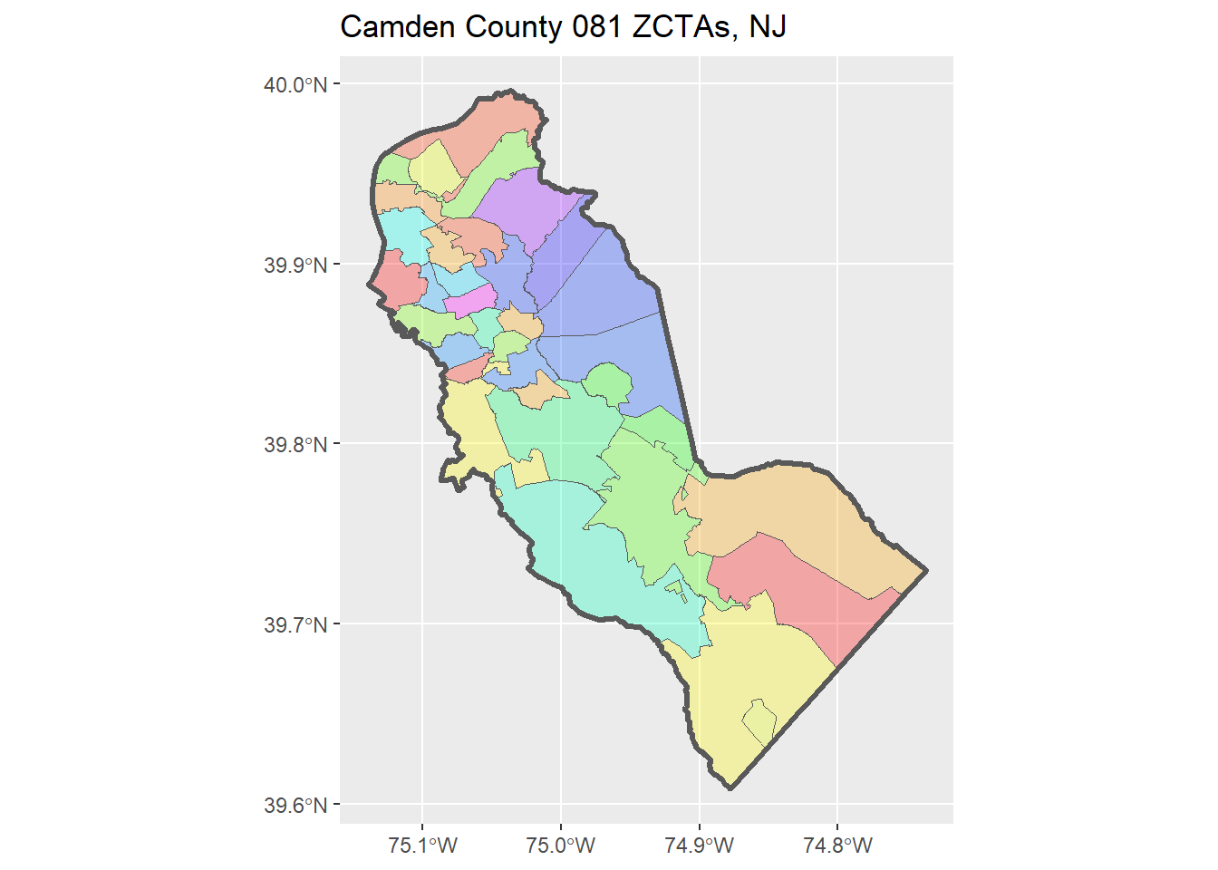

Save a local copy:

saveRDS(camden_zcta20_sf, file.path(my_data_dir, "camden_zcta20_sf.Rds"))

3 Import Data from ArcGIS

Many state and local government agencies share GIS data using ArcGIS resources. Quite often, they use a product called ArcGIS Hub to make base layers available with the public thru an open data portal. Examples:

• Camden County ArcGIS Open Data Hub
  
• New Jersey Office of GIS

Finding Open Data

You can also discover state and local data open sources, including non-ESRI platforms, at: https://www.opendatanetwork.com/.

We will use the arcgislayers package to bring these layers into R. Because these layers have been made publicly available, we do not need an ArcGIS account to download them.

3.1 Setup

The easiest way to install arcgislayers and a couple of other packages that are needed behind the scenes is to install the arcgis ‘meta package’.

# install.packages("arcgis")
library(arcgislayers)

3.2 Import Municipality Boundaries

The Camden County Department of Public Works publishes municipalities boundaries on their Open Data Hub. You can see the description page here:

https://camdencountynj-ccdpw.opendata.arcgis.com/datasets/9bea5658edfa490c9d00f98fd9efb6d6_0/

To import it into R, we need to find the FeatureServer URL:

1. on the description page above, click ‘View Full Details’
2. scroll down > ‘Open in ArcGIS Online’
3. Take note of the sublayer(s) in this Feature Layer
4. scroll down > copy URL

https://services3.arcgis.com/JGF6qCAQFbROcocK/arcgis/rest/services/CamdenCountyMunicipalLayer/FeatureServer

Now we’re ready to import it:

camden_munip22_url <- "https://services3.arcgis.com/JGF6qCAQFbROcocK/arcgis/rest/services/CamdenCountyMunicipalLayer/FeatureServer"

## Step 1. Open the URL to get the FeatureServer connection
camden_munip22_ftsrv <- arcgislayers::arc_open(camden_munip22_url)
camden_munip22_ftsrv

<FeatureServer <1 layer, 0 tables>>
CRS: 26918
Capabilities: Query,Sync
  0: CamdenCounty_Municipal2022 (esriGeometryPolygon)

Next, we select the (sub)layer we want (in this case there is only one).

Tip

The indices of Feature Layers available from a Feature Server start at 0.

camden_munip22_ftlyr <- arcgislayers::get_layer(camden_munip22_ftsrv, 0)
camden_munip22_ftlyr

<FeatureLayer>
Name: CamdenCounty_Municipal2022
Geometry Type: esriGeometryPolygon
CRS: 26918
Capabilities: Query,Sync

Next, we import our chosen Feature Layer into R with arc_select():

camden_munip22_prj_sf <- arcgislayers::arc_select(camden_munip22_ftlyr) 

Registered S3 method overwritten by 'jsonify':
  method     from    
  print.json jsonlite

camden_munip22_prj_sf

arc_select() returns a sf object, but it is in a different CRS than the layers from the US Census.

camden_munip22_prj_sf |> sf::st_crs()

Coordinate Reference System:
  User input: EPSG:26918 
  wkt:
PROJCRS["NAD83 / UTM zone 18N",
    BASEGEOGCRS["NAD83",
        DATUM["North American Datum 1983",
            ELLIPSOID["GRS 1980",6378137,298.257222101,
                LENGTHUNIT["metre",1]]],
        PRIMEM["Greenwich",0,
            ANGLEUNIT["degree",0.0174532925199433]],
        ID["EPSG",4269]],
    CONVERSION["UTM zone 18N",
        METHOD["Transverse Mercator",
            ID["EPSG",9807]],
        PARAMETER["Latitude of natural origin",0,
            ANGLEUNIT["degree",0.0174532925199433],
            ID["EPSG",8801]],
        PARAMETER["Longitude of natural origin",-75,
            ANGLEUNIT["degree",0.0174532925199433],
            ID["EPSG",8802]],
        PARAMETER["Scale factor at natural origin",0.9996,
            SCALEUNIT["unity",1],
            ID["EPSG",8805]],
        PARAMETER["False easting",500000,
            LENGTHUNIT["metre",1],
            ID["EPSG",8806]],
        PARAMETER["False northing",0,
            LENGTHUNIT["metre",1],
            ID["EPSG",8807]]],
    CS[Cartesian,2],
        AXIS["(E)",east,
            ORDER[1],
            LENGTHUNIT["metre",1]],
        AXIS["(N)",north,
            ORDER[2],
            LENGTHUNIT["metre",1]],
    USAGE[
        SCOPE["Engineering survey, topographic mapping."],
        AREA["North America - between 78°W and 72°W - onshore and offshore. Canada - Nunavut; Ontario; Quebec. United States (USA) - Connecticut; Delaware; Maryland; Massachusetts; New Hampshire; New Jersey; New York; North Carolina; Pennsylvania; Virginia; Vermont."],
        BBOX[28.28,-78,84,-72]],
    ID["EPSG",26918]]

We can ‘unproject’ it to NAD83 with sf::st_transform():

camden_munip22_sf <- camden_munip22_prj_sf |> 
  sf::st_transform(4269)

Now we’re ready to plot it with the county boundary:

ggplot(camden_munip22_sf) + 
  geom_sf() + 
  geom_sf(data = camden_bnd_sf, fill = NA, lwd = 1.2) +
  labs(title = "Camden County Municipalities, 2022") +
  theme_light()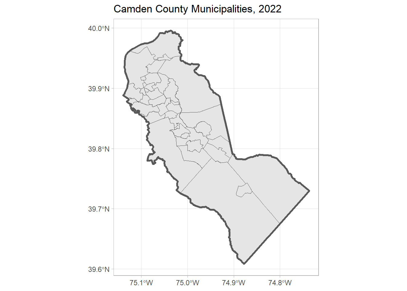

Save a local copy:

saveRDS(camden_munip22_sf, file.path(my_data_dir, "camden_munip22_sf.Rds"))

3.3 Import Wards

Using a similar process we can import the Wards for Camden County from the NJ Office of GIS Open Data Hub.

After you find the URL for the Feature Server, we can get the layer:

nj_wards20_url <- "https://services2.arcgis.com/XVOqAjTOJ5P6ngMu/arcgis/rest/services/Ward_Boundaries_for_New_Jersey/FeatureServer"
nj_wards20_ftsrv <- arc_open(nj_wards20_url)
nj_wards20_ftsrv

<FeatureServer <1 layer, 0 tables>>
CRS: 3424
Capabilities: Query,Extract
  0: Govt_admin_ward (esriGeometryPolygon)

nj_wards20_ftlyr <- get_layer(nj_wards20_ftsrv, 0)
nj_wards20_ftlyr

<FeatureLayer>
Name: Govt_admin_ward
Geometry Type: esriGeometryPolygon
CRS: 3424
Capabilities: Query,Extract

nj_wards20_ftlyr contains the wards for the entire state of NJ, but we only need the Wards for Camden County. We can let the server do the filtering for us by using additional arguments in arc_select().

First we need to construct a query expression we can use for the where argument. Let’s view the fields:

arcgislayers::list_fields(nj_wards20_ftlyr)

We see a field called COUNTY that might work:

camden_wards20_prj_sf <- arcgislayers::arc_select(nj_wards20_ftlyr, where = "COUNTY = 'Camden'") 
camden_wards20_prj_sf

head(camden_wards20_prj_sf)

Aside from the projection, this looks good-to-go.

camden_wards20_sf <- camden_wards20_prj_sf |> 
  st_transform(4269)

Plot:

ggplot(camden_wards20_sf) + 
  geom_sf() + 
  geom_sf(data = camden_bnd_sf, fill = NA, lwd = 1.2) +
  labs(title = "Camden County Wards, 2020") +
  theme_light()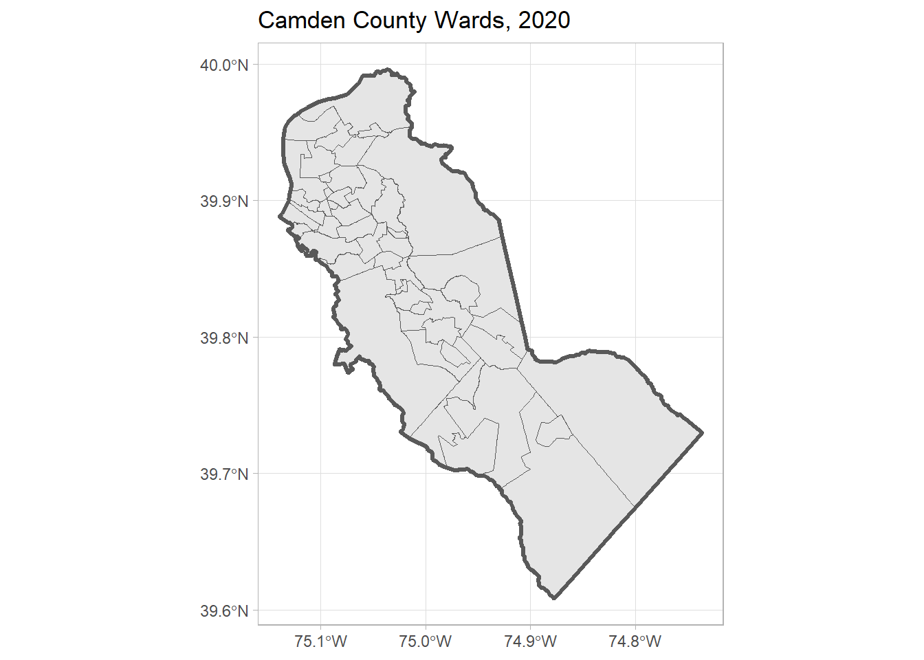

And save:

saveRDS(camden_wards20_sf, file.path(my_data_dir, "camden_wards20_sf.Rds"))

3.4 CHALLENGE

Import the Camden County Schools, and plot them. (Solution)

## Your answer here

4 DONE!

Remember to save your Quarto document. If you’re working on Posit Cloud, you can down a copy from the File Pane > More > Export.