Analyzing Voter Turnout Data with R
Part 1: Data Wrangling and Geospatial Fundamentals
![]()
Data
for Democracy, Fall 2024
Andy Lyons
![]()
Data
for Democracy, Fall 2024
Andy Lyons
![]()
Homerange and spatial-temporal pattern analysis for wildlife tracking
data
http://tlocoh.r-forge.r-project.org/
Data management utilities for drone mapping
https://ucanr-igis.github.io/uasimg/

Bring climate data from Cal-Adapt into R using the API
https://ucanr-igis.github.io/caladaptr/

Compute degree days in R
https://ucanr-igis.github.io/degday/
Chill Portions Under Climate Change Calculator
https://ucanr-igis.shinyapps.io/chill/
Drone Mission Planner for Reforestation Monitoring Protocol
https://ucanr-igis.shinyapps.io/uav_stocking_survey/
Stock Pond Volume Calculator
https://ucanr-igis.shinyapps.io/PondCalc/
Pistachio Nut Growth Calculator
https://ucanr-igis.shinyapps.io/pist_gdd/
The keys to R’s superpowers are functions! There are four things you need to know to use a function:

|
Finding the right R function, half the battle is. - Jedi MasteR Yoda |

|
Ask your friends
Ask Google
Cheatsheets!
Every function has a help page. To get to it enter ?
followed by the name of the function (without parentheses):
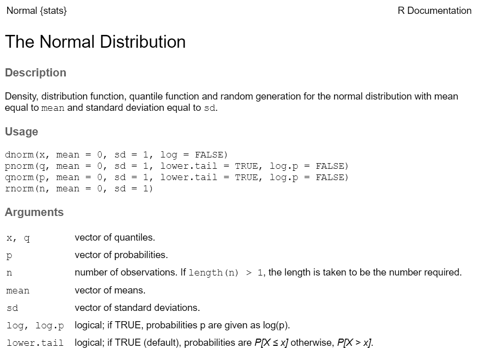
Most functions take arguments. Arguments can be required or optional (i.e. have a default value).
See the function’s help page to determine which arguments are expected. Example:
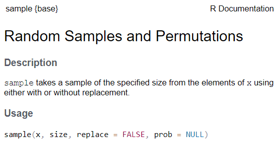
x and size have no default value → they are
required
replace and prob have default values → they
are optional
All arguments have names. You can explicitly name arguments when calling a function as follows:
Benefits of naming your arguments:
But you can omit argument names if you pass them in the order expected and don’t skip any.

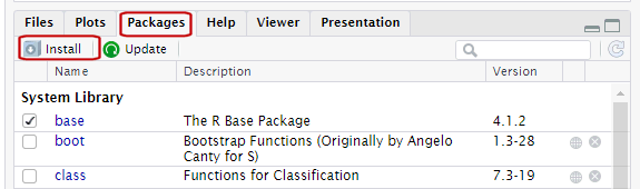
Packages are what R calls extensions or add-ons.
Three simple steps to use the functions in a package:
Figure out which package you need
Install (i.e., download) it (just once)

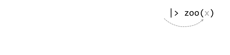
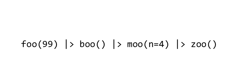
Piping syntax is an alternative way of writing arguments into functions.
With piping, you use the pipe operator |> (or %>%) to ‘feed’ the result of one function into the next function.
Piping allows the results of one function to be passed as the first argument of the next function. Hence a series of commands to be written like a sentence.
Consider the expression:
zoo(moo(boo(foo(99)),n=4))


Occasionally two or more packages will have different functions that
use the same name. 
When this happens, R will use whichever one was loaded first.
Best practice: use the package name and the :: reference
to specify which package a function is from.
When you use the package_name::function_name
syntax, you don’t actually have to first load the package with
library().
Resolving Name Conflicts with the conflicted
Package
When you call a function that exists in multiple packages, R uses whichever package was loaded first.
The conflicted package helps you avoid problems with
duplicate function names, by specifying which one to prioritize no
matter what order they were loaded.
Whatever is needed to get your data frame ready
for the function(s) you want to use for analysis and visualization.
also called data munging, manipulation, transformation, etc.
Often includes one or more of:
dplyr![]()
An alternative (usually better) way to wrangle data frames than base R.
Part of the tidyverse.
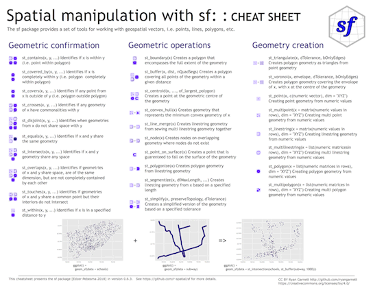
Best way to familiarize yourself - explore the cheat sheet:
![]()
sf![]()
sf is a popular package for working
with vector geospatial data
sf stands for ‘simple feature’, which is a standard
(developed by the Open Geospatial Consortium) for storing various
geometry types in a hierarchical data model.
A ‘feature’ is just a representation of a thing in the real world (e.g. a building, a city, ).
Package features:
sf functionsst_)|> pipe friendly!
How do we squish a round planet onto flat maps / screens?
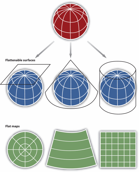
There are 1000s of projections!
Each one has an EPSG number.
The more generic term for projections is Coordinate Reference System (CRS).
CRS also includes ‘unprojected’ geographic coordinates (longitude & latitude).
Projections are particularly important in R whenever you want to:
tigris![]()
The tigris
package (by Kyle Walker) provides functions to download Shapefiles from
the US Census Bureau.
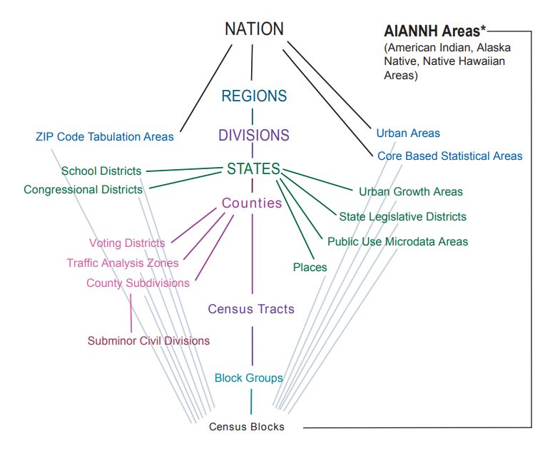
tigris features:
cb = TRUE) to
mask areas by coastlines & water features
tigris only downloads the geometries. To get census data
as spatial objects, see tidyCensus.
tigris functions** where available
Most of these functions have arguments you can use to limit the results to specific state(s) and/or county(s).
arcgislayers![]()
arcgislayers
package (by Josiah Parry) provides an R interface to work with ArcGIS
services on ArcGIS.com and ArcGIS Portal using the API
Key functions include:
This is really useful, because:
Go to the “item details” page on ArcGIS.com for the layer you want.
Find the URL for the FeatureServer or MapServer.
Create a connection to the FeatureServer or MapServer (with
arc_open()).
Use get_layer() to create a connection to the
specific FeatureLayer you want to import.
Import the layer using arc_select(), providing an
attribute and/or spatial query expression if needed.
The layer comes into R as a simple feature (sf) object
library(sf)
library(arcgislayers)

## URL for a pubicly available Feature Server
counties_featsrv_url <- "https://services.arcgis.com/P3ePLMYs2RVChkJx/ArcGIS/rest/services/USA_Counties_Generalized_Boundaries/FeatureServer/"

## Create a FeatureServer object
counties_featsrv_fs <- arc_open(counties_featsrv_url)
counties_featsrv_fs
## <FeatureServer <1 layer, 0 tables>>
## CRS: 4326
## Capabilities: Query,Extract
## 0: USA Counties - Generalized (esriGeometryPolygon)## # A data frame: 1 × 9
## id name parentLayerId defaultVisibility subLayerIds minScale maxScale
## * <int> <chr> <int> <lgl> <lgl> <int> <int>
## 1 0 USA Count… -1 TRUE NA 0 0
## # ℹ 2 more variables: type <chr>, geometryType <chr>## Create a FeatureLayer object
counties_featsrv_fl <- arcgislayers::get_layer(counties_featsrv_fs, id = 0)
counties_featsrv_fl## <FeatureLayer>
## Name: USA Counties - Generalized
## Geometry Type: esriGeometryPolygon
## CRS: 4326
## Capabilities: Query,Extract## View the fields in the attribute table
## list_fields(counties_featsrv_fl) |> View()
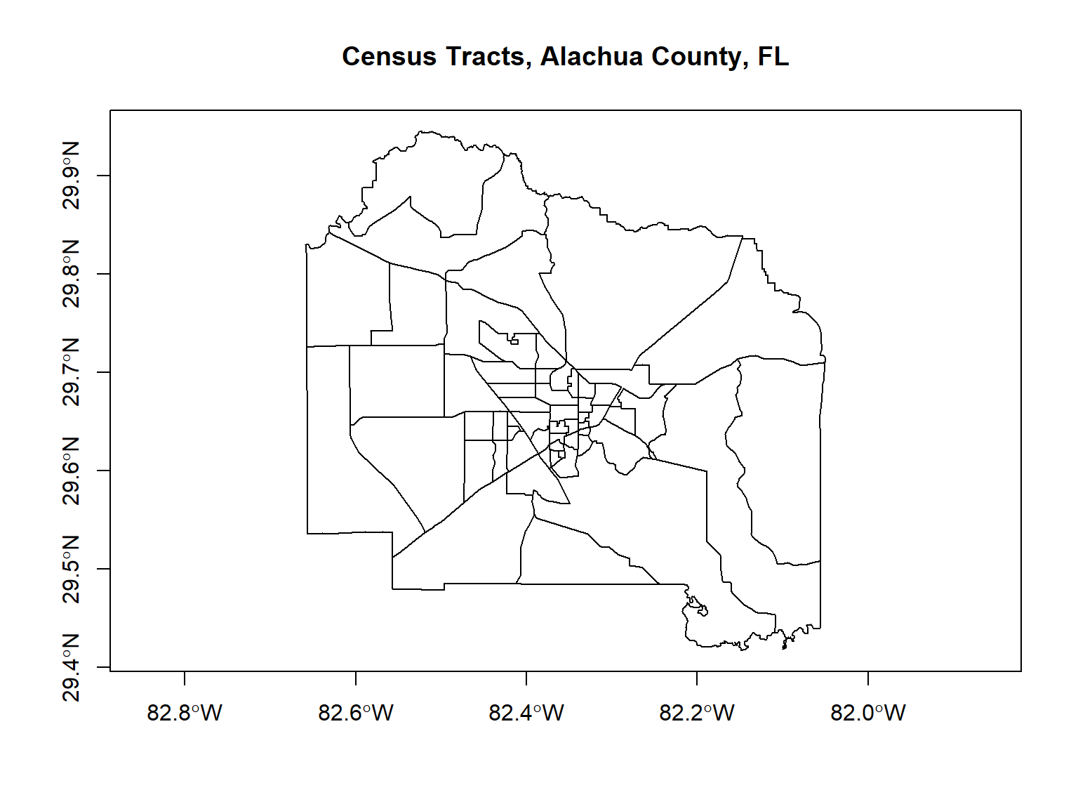
## Import just the Florida Counties
fl_counties_sf <- arc_select(counties_featsrv_fl, where = "STATE_FIPS = '12'")
plot(fl_counties_sf$geometry, axes = TRUE)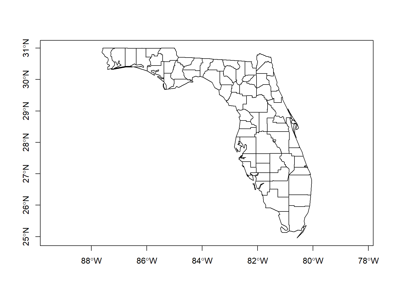
To import non-public data from ArcGIS online / portal, you need to authenticate by:
Create a Developer Auth Credentials (i.e., a service account) by logging into ArcGIS.com > Content > Add Content > New Developer Auth Credentials).
Feed your ‘client id’ and ‘client secret’ into
arcgisutils::auth_code() or
arcgisutils::auth_client() to generate a temporary
token.
Pass the token to arc_open(),
arc_select(), and other functions where needed.
Refresh the token when needed with
arcgisutils::refresh_token().
ggplot2 is an extremely popular plotting package for R.
Plots are constructed using the ‘grammar of graphics’ metaphor.
Load Palmer Penguins data frame:
## # A tibble: 6 × 8
##   species island    bill_length_mm bill_depth_mm flipper_length_mm body_mass_g
##   <fct>   <fct>              <dbl>         <dbl>             <int>       <int>
## 1 Adelie  Torgersen           39.1          18.7               181        3750
## 2 Adelie  Torgersen           39.5          17.4               186        3800
## 3 Adelie  Torgersen           40.3          18                 195        3250
## 4 Adelie  Torgersen           NA            NA                  NA          NA
## 5 Adelie  Torgersen           36.7          19.3               193        3450
## 6 Adelie  Torgersen           39.3          20.6               190        3650
## # ℹ 2 more variables: sex <fct>, year <int>
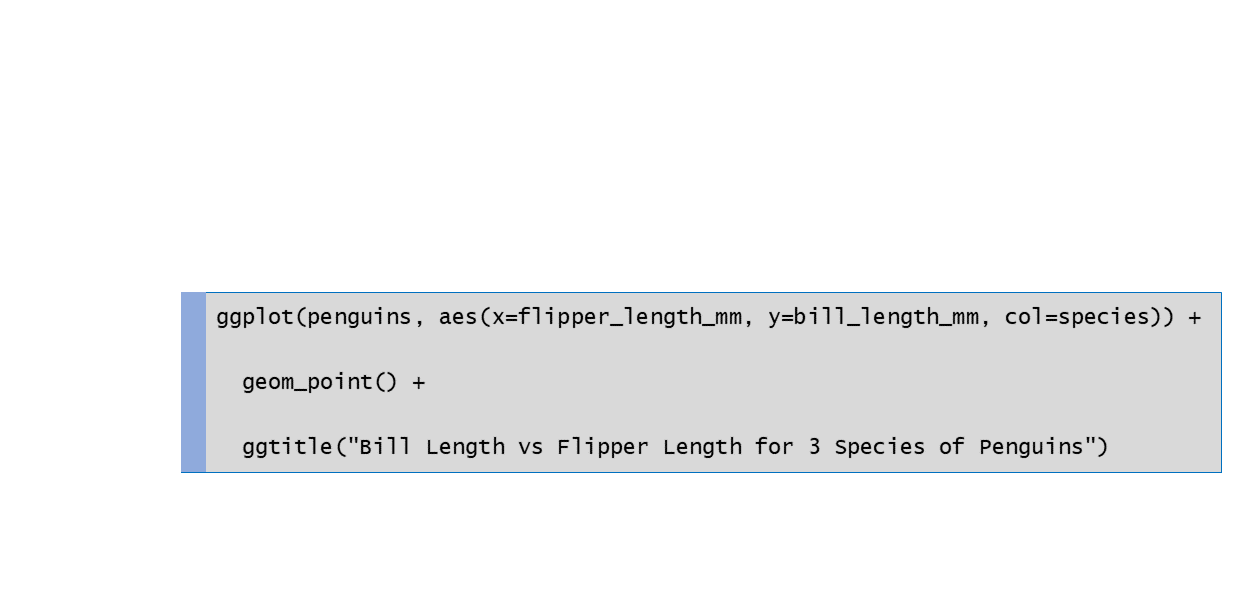
Use ggplot to make a scatter plot:
library(ggplot2)
ggplot(penguins, aes(x = flipper_length_mm, y = bill_length_mm, color = species)) +
  geom_point() +
  ggtitle("Bill Length vs Flipper Length for 3 Species of Penguins")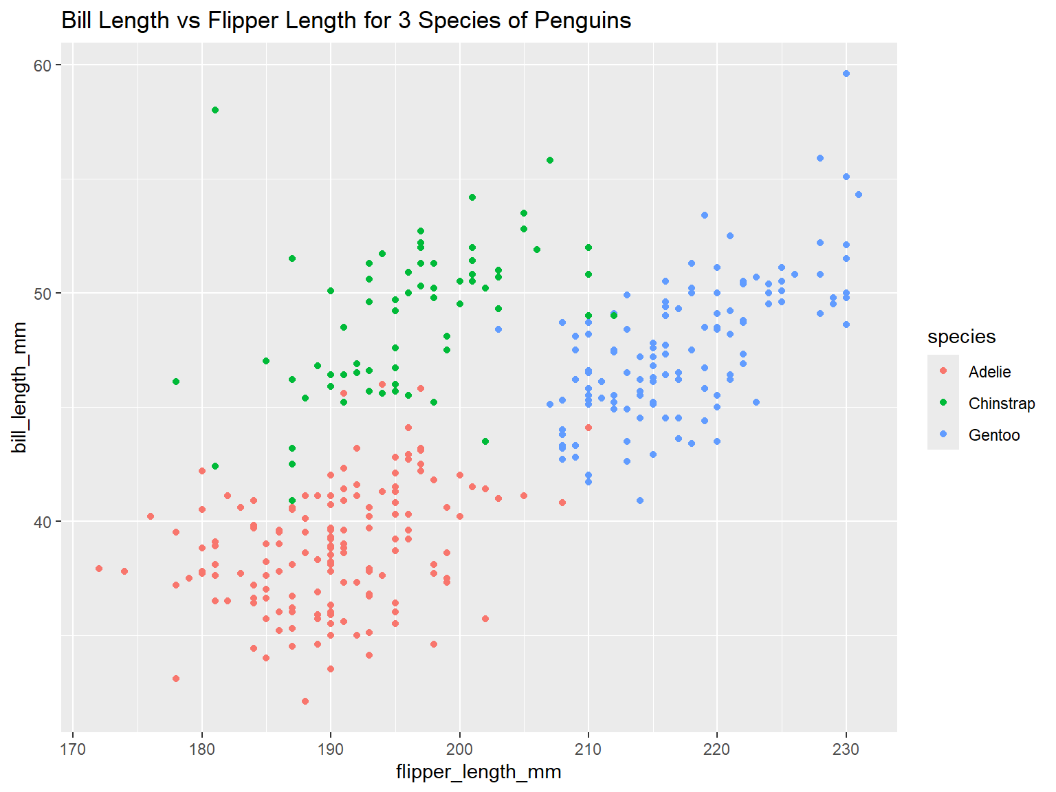
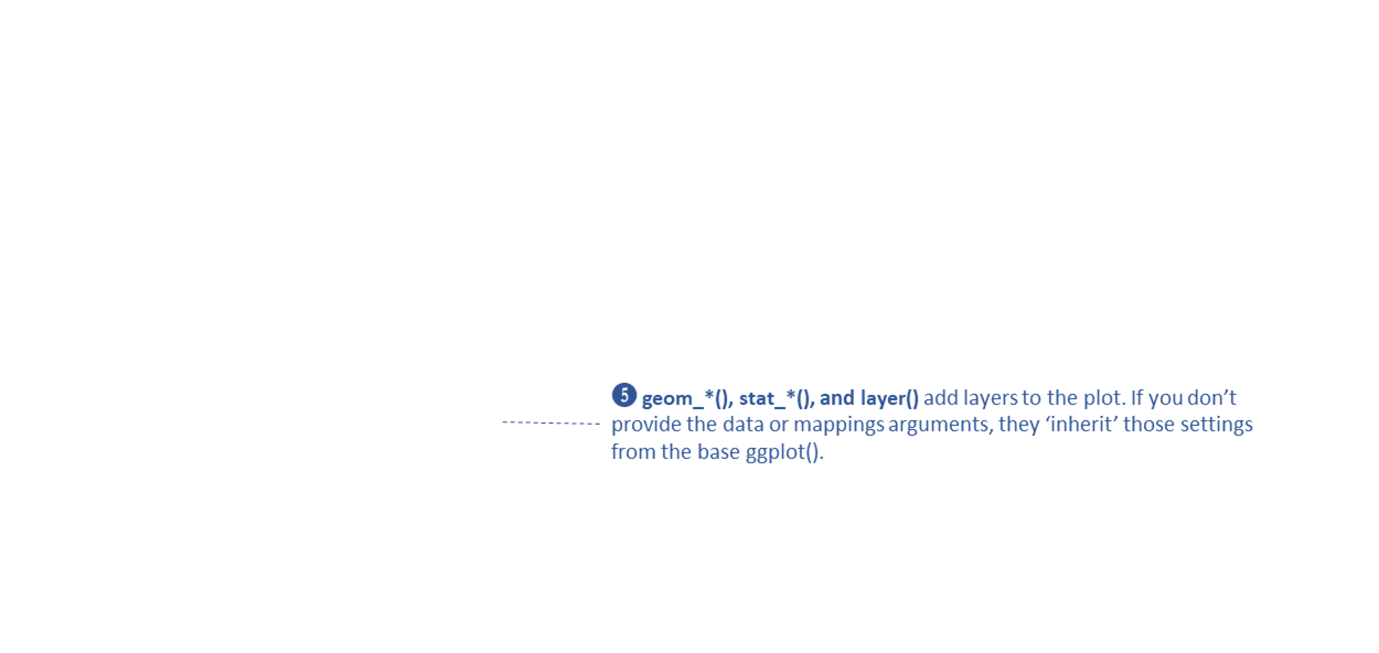
geom_xxxx() functions draw layers on the plot
canvas
drawn from the bottom up
some common geoms:
geom_point(col = pop_size)
geom_point(col = “red”)
visual properties are inherited (from
aes())
each geom has default color palettes and legend settings
In the example below, note where geom_boxplot() gets its
visual properties:
aes()ggplot(penguins, aes(x = species, y = bill_length_mm)) +
geom_boxplot(color = "navy", fill = "yellow", size = 1.5)## Warning: Removed 2 rows containing non-finite outside the scale range
## (`stat_boxplot()`).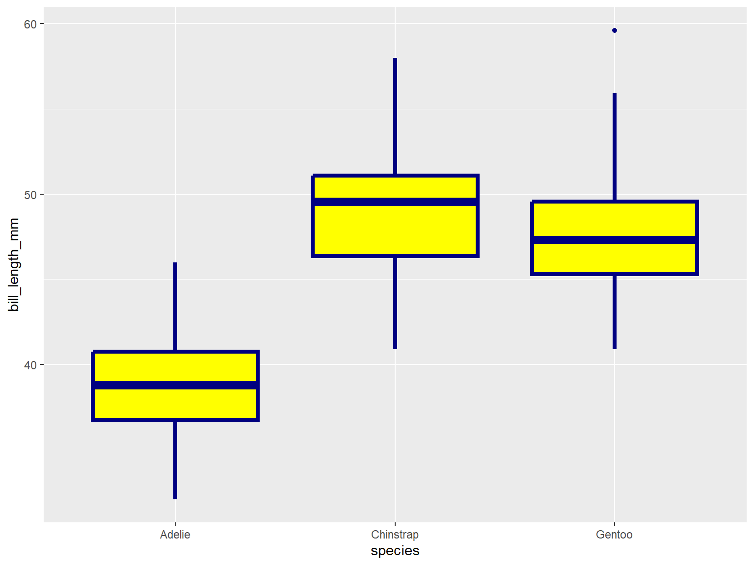
geom_xxxx() functions can also be used to add other
graphic elements:
ggplot(penguins, aes(x = species, y = bill_length_mm)) +
geom_boxplot(color = "navy", fill = "yellow", size = 1.5) +
geom_hline(yintercept = 43.9, linewidth = 3, color="red") +
geom_label(x = 3, y = 58, label = "Gentoo penguins \n are just the best!")## Warning: Removed 2 rows containing non-finite outside the scale range
## (`stat_boxplot()`).
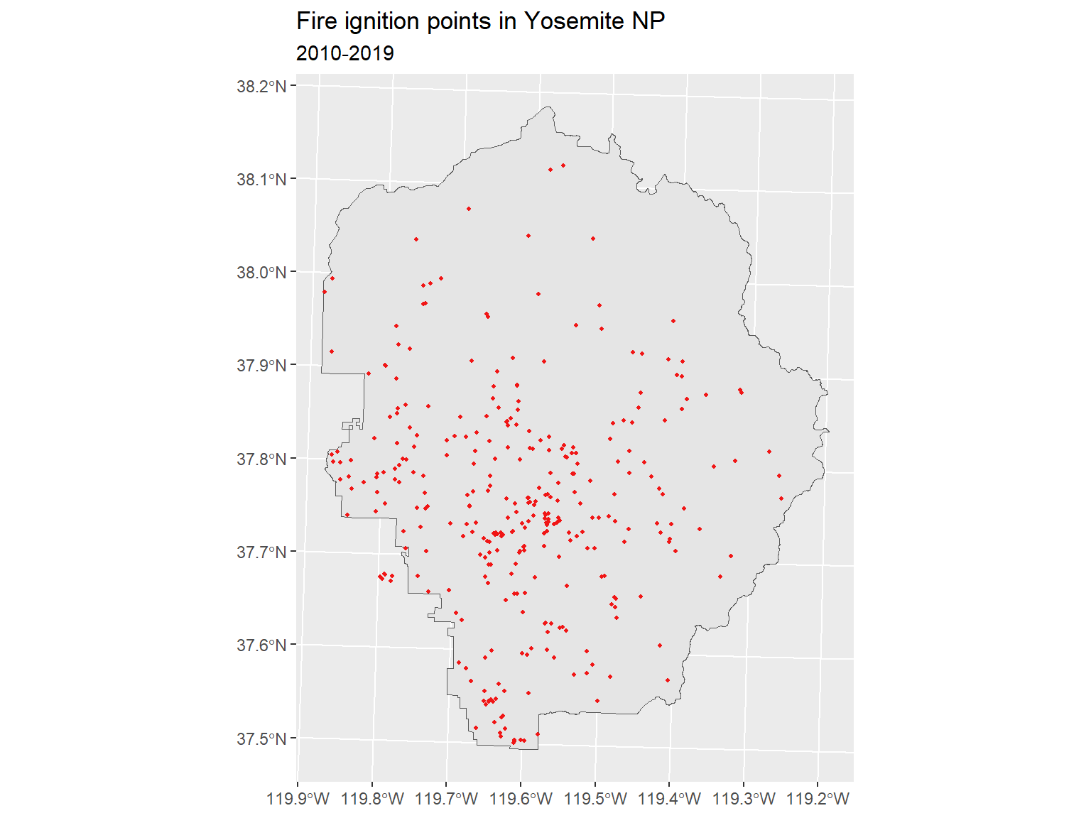
library(sf)
epsg_utm11n_nad83 <- 26911

## Park boundary
yose_bnd_utm <- sf::st_read(dsn="./data", layer="yose_boundary", quiet=TRUE) |>
  st_transform(epsg_utm11n_nad83)

## Fire ignition points
yose_firehist_pts_utm <- sf::st_read("./data/yose_firehistory.gdb", "YNP_FireHistoryPoints", quiet=TRUE) |>
  st_transform(epsg_utm11n_nad83)
library(ggplot2)
library(dplyr)

ggplot() +
  geom_sf(data = yose_bnd_utm) +
  geom_sf(data = yose_firehist_pts_utm |> filter(DECADE >= 2010), color="#f01616", shape=16, cex=0.7) +
  labs(title = "Fire ignition points in Yosemite NP", subtitle = "2010-2019")