Analyzing Voter Turnout Data with R
Part 2: Joining Tabular Data to Shapefiles
![]()
Data
for Democracy, Fall 2024
Andy Lyons
![]()
Data
for Democracy, Fall 2024
Andy Lyons
![]()
https://redistrictingdatahub.org/
The nonpartisan Redistricting Data Hub provides individuals, good government organizations, and community groups the data, resources, and knowledge to participate effectively in the redistricting process.

![]()
![]()

These packages allow you to:
Example:
\*.shp,
\*.shx, \*.prj, \*.dbf,
etc.
st_read(dsn, layer)
dsn - directory, or shp filename
layer - shp filename (minus .shp), or omitted
library(sf)
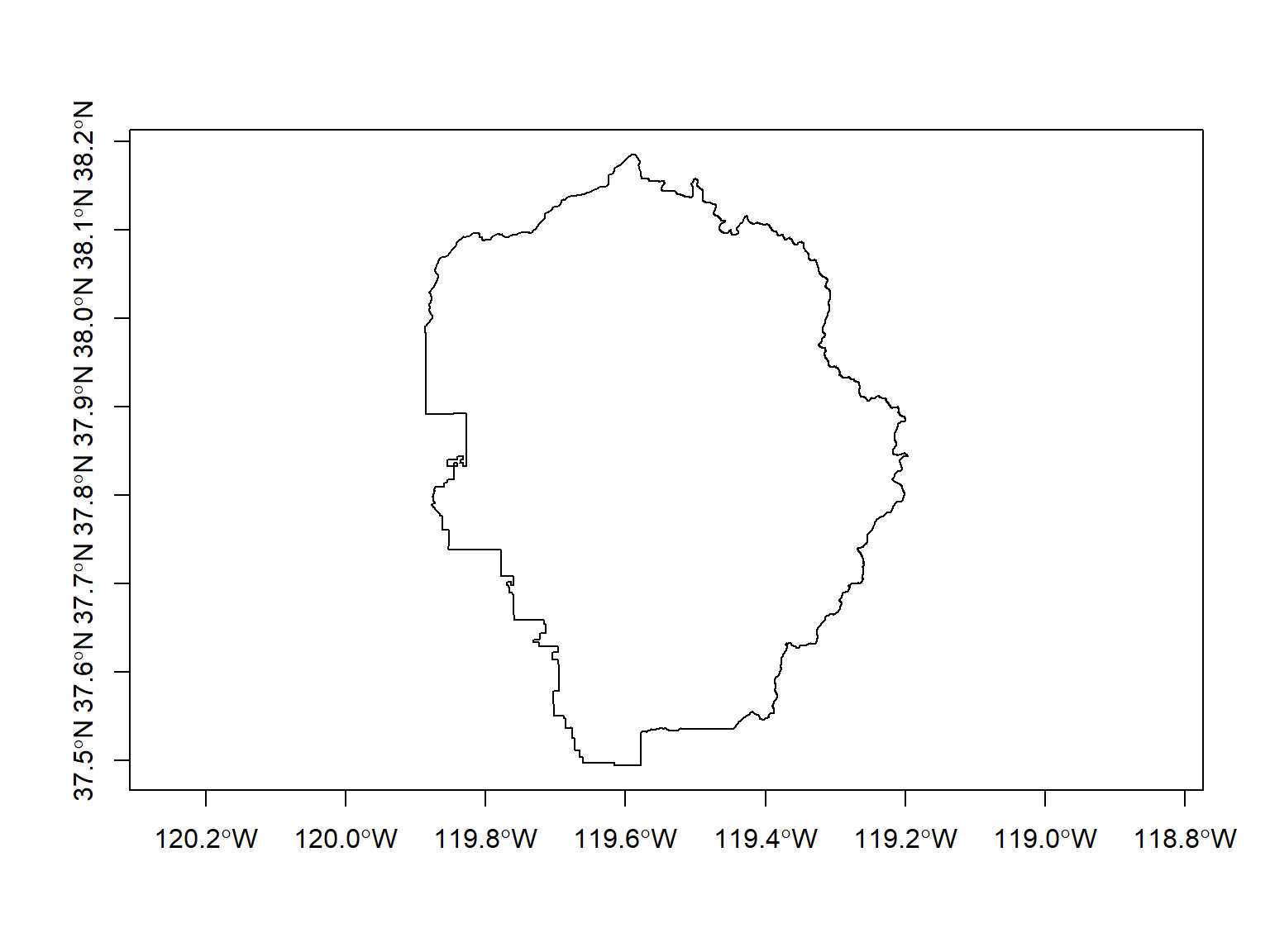
yose_bnd_ll <- st_read(dsn="./data", layer="yose_boundary")
## This would also work:
## yose_bnd_ll <- st_read(dsn="./data/yose_boundary.shp")
View contents:
## Simple feature collection with 1 feature and 11 fields
## Geometry type: POLYGON
## Dimension:     XY
## Bounding box:  xmin: -119.8864 ymin: 37.4947 xmax: -119.1964 ymax: 38.18515
## Geodetic CRS:  North_American_Datum_1983
##   UNIT_CODE
## 1      YOSE
##                                                                             GIS_NOTES
## 1 Lands - http://landsnet.nps.gov/tractsnet/documents/YOSE/METADATA/yose_metadata.xml
##                UNIT_NAME  DATE_EDIT STATE REGION GNIS_ID     UNIT_TYPE
## 1 Yosemite National Park 2016-01-27    CA     PW  255923 National Park
##   CREATED_BY                                               METADATA PARKNAME
## 1      Lands http://nrdata.nps.gov/programs/Lands/YOSE_METADATA.xml Yosemite
##                         geometry
## 1 POLYGON ((-119.8456 37.8327...
Plot:
| join data frames on a column | left_join(), right_join(), inner_join() |
| stack data frames | bind_rows() |
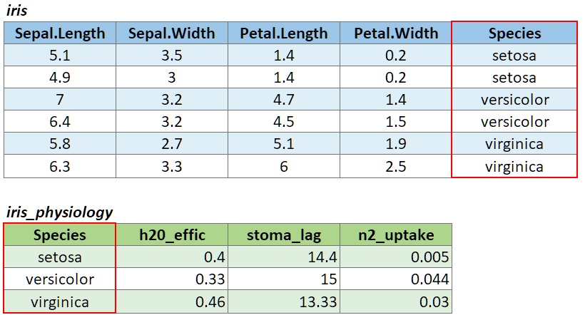
To join two data frames based on a common column, you can use:
left_join(x, y, by)
where x and y are data frames, and by is the name of a column they have in common.
If there is only one column in common, and if it has the same name in both data frames, you can omit the by argument.
If the common column is named differently in the two data frames, you can deal with that by passing a named vector as the by argument. See below.
To illustrate a table join, we’ll first import a csv with some fake data about the genetics of different iris species:
# Create a data frame with additional info about the three IRIS species
iris_genetics <- data.frame(Species=c("setosa", "versicolor", "virginica"),
                          num_genes = c(42000, 41000, 43000),
                          prp_alles_recessive = c(0.8, 0.76, 0.65))

iris_genetics
## Species num_genes prp_alles_recessive
## 1 setosa 42000 0.80
## 2 versicolor 41000 0.76
## 3 virginica 43000 0.65We can join these additional columns to the iris data frame with
left_join():
##    Sepal.Length Sepal.Width Petal.Length Petal.Width Species num_genes
## 1           5.1         3.5          1.4         0.2  setosa     42000
## 2           4.9         3.0          1.4         0.2  setosa     42000
## 3           4.7         3.2          1.3         0.2  setosa     42000
## 4           4.6         3.1          1.5         0.2  setosa     42000
## 5           5.0         3.6          1.4         0.2  setosa     42000
## 6           5.4         3.9          1.7         0.4  setosa     42000
## 7           4.6         3.4          1.4         0.3  setosa     42000
## 8           5.0         3.4          1.5         0.2  setosa     42000
## 9           4.4         2.9          1.4         0.2  setosa     42000
## 10          4.9         3.1          1.5         0.1  setosa     42000
##    prp_alles_recessive
## 1                  0.8
## 2                  0.8
## 3                  0.8
## 4                  0.8
## 5                  0.8
## 6                  0.8
## 7                  0.8
## 8                  0.8
## 9                  0.8
## 10                 0.8
If you need to join tables on multiple columns, add additional column
names to the by argument.
Join columns must be the same data type (i.e., both numeric or both character).
There are several variants of left_join(), the most
common being right_join() and
inner_join(). See help for details.
If the join column is named differently in the two tables, you can
pass a named character vector as the by argument. A named
vector is a vector whose elements have been assigned names. You can
construct a named vector with c().
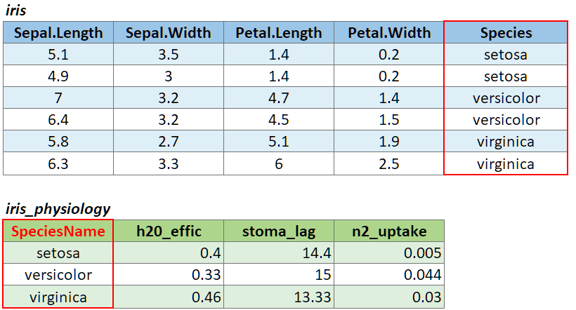
For example if the join column was named ‘SpeciesName’ in x, and just ‘Species’ in y, your expression would be:
left_join(x, y, by = c("SpeciesName" = "Species"))

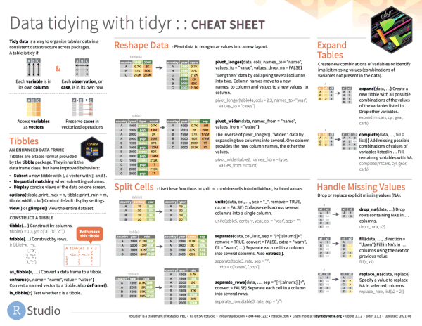
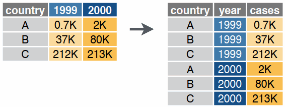
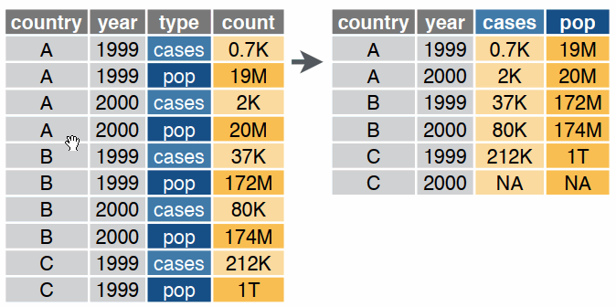
Reshaping data includes:
The go-to Tidyverse package for reshaping data frames is tidyr