Common Manipulations for sf Objects

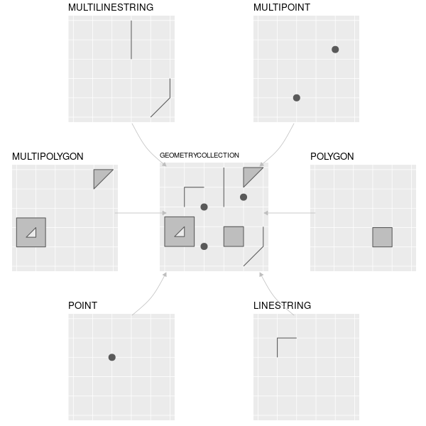
simple features is an ISO standard for storing and accessing spatial data. It is widely adopted in spatial databases, open source formats like GeoJSON, GIS software, tools, etc.
sf employs a standard called “Well Known Text” (WKT) to encode the geometry. WKT is a very simple written representation of the ‘connect-the-dots’ vector data model.
| Geometry | Sample WKT |
|---|---|
| point | POINT (2 4) |
| multipoint | MULTIPOINT (2 2, 3 3, 3 2) |
| linestring | LINESTRING (0 3, 1 4, 2 3) |
| polygon | POLYGON ((1 0, 3 4, 5 1, 1 0)) |
Import the Yosemite points-of-interest Shapefile.
library(sf)
## Import the Yosemite Points-of-Interest Shapefile
yose_poi_utm <- st_read(dsn="./data", layer="yose_poi")
## View column names in the attribute table
names(yose_poi_utm)
## Plot the points
plot(yose_poi_utm |> st_geometry(), pch=16, asp=1, cex=0.5, axes=TRUE)## Reading layer `yose_poi' from data source `D:\Workshops\R-Spatial\rspatial_mod\outputs\rspatial_bgs24\exercises\data' using driver `ESRI Shapefile'
## Simple feature collection with 2720 features and 30 fields
## Geometry type: POINT
## Dimension: XY
## Bounding box: xmin: 246416.2 ymin: 4153717 xmax: 301510.7 ymax: 4208419
## Projected CRS: NAD83 / UTM zone 11N
## [1] "OBJECTID" "POINAME" "POIALTNAME" "POILABEL" "POIFEATTYP" "POITYPE" "UNITCODE" "UNITNAME" "GROUPCODE" "REGIONCODE" "ISEXTANT" "MAPMETHOD"
## [13] "MAPSOURCE" "SRCESCALE" "SOURCEDATE" "XYERROR" "LOCATIONID" "ASSETID" "NOTES" "DISTRIBUTE" "RESTRICTIO" "CREATEDATE" "CREATEUSER" "EDITDATE"
## [25] "EDITUSER" "FEATUREID" "GEOMETRYID" "PLACESID" "GlobalID" "TAGS" "geometry"

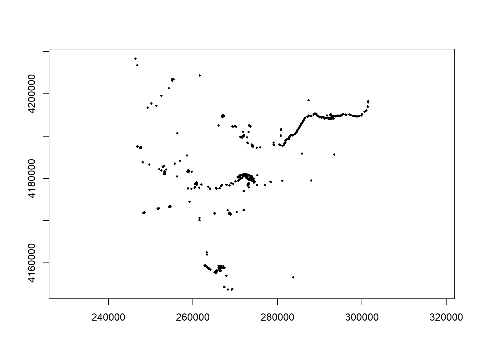
Take a closer look at the geometry column:
## [1] "sfc_POINT" "sfc"
## Simple feature collection with 6 features and 0 fields
## Geometry type: POINT
## Dimension: XY
## Bounding box: xmin: 260859.4 ymin: 4153717 xmax: 270931.1 ymax: 4179771
## Projected CRS: NAD83 / UTM zone 11N
## geometry
## 1 POINT (260859.4 4178493)
## 2 POINT (264115.4 4158415)
## 3 POINT (268276.8 4153717)
## 4 POINT (268620.1 4178344)
## 5 POINT (269052.6 4178870)
## 6 POINT (270931.1 4179771)
The geometry column of a sf object does not have to be called ‘geometry’. You can view the column name by running attr(x, "sf_column") where x is a sf object.
The features in a sf object can be a mix of points, lines, and polyons. The data class of the geometry column is therefore sfc (simple features collection).

Bounding box
It’s often useful to view the metadata of a sf object. You can get the bounding box (aka extent) with st_bbox().
Coordinates
To extract the coordinates of a sf object as a matrix, use st_coordinates().
Projections are particularly important whenever you want to:
The more generic term for projections as is Coordinate Reference System (CRS).
CRS also includes unprojected geographic coordinates (longitude & latitude).
A CRS has three parts:
All sf objects are able to store projection info.
st_read() imports the CRS info from standard GIS file formats
st_crs() creates, views, or assigns the CRS
st_transform() (re)projects sf objects into a different crs
The sf package uses the PROJ.4 library for established CRS. It provides two ways to specify a known projection:
EPSG codes were developed by the European Petroluem Survey Group.
The following are equivalent:
If you happen to know the proj4string, you can use it also
## Coordinate Reference System:
## User input: +proj=utm +zone=10 +ellps=GRS80 +datum=NAD83 +units=m +no_defs
## wkt:
## PROJCRS["unknown",
## BASEGEOGCRS["unknown",
## DATUM["North American Datum 1983",
## ELLIPSOID["GRS 1980",6378137,298.257222101,
## LENGTHUNIT["metre",1]],
## ID["EPSG",6269]],
## PRIMEM["Greenwich",0,
## ANGLEUNIT["degree",0.0174532925199433],
## ID["EPSG",8901]]],
## CONVERSION["UTM zone 10N",
## METHOD["Transverse Mercator",
## ID["EPSG",9807]],
## PARAMETER["Latitude of natural origin",0,
## ANGLEUNIT["degree",0.0174532925199433],
## ID["EPSG",8801]],
## PARAMETER["Longitude of natural origin",-123,
## ANGLEUNIT["degree",0.0174532925199433],
## ID["EPSG",8802]],
## PARAMETER["Scale factor at natural origin",0.9996,
## SCALEUNIT["unity",1],
## ID["EPSG",8805]],
## PARAMETER["False easting",500000,
## LENGTHUNIT["metre",1],
## ID["EPSG",8806]],
## PARAMETER["False northing",0,
## LENGTHUNIT["metre",1],
## ID["EPSG",8807]],
## ID["EPSG",16010]],
## CS[Cartesian,2],
## AXIS["(E)",east,
## ORDER[1],
## LENGTHUNIT["metre",1,
## ID["EPSG",9001]]],
## AXIS["(N)",north,
## ORDER[2],
## LENGTHUNIT["metre",1,
## ID["EPSG",9001]]]]
4326. Geographic, WGS84 (default for lon/lat)
4269. Geographic, NAD83 (USA Fed agencies like Census)
5070. USA Contiguous Albers Equal Area Conic
3310. CA ALbers Equal Area
32610. UTM Zone 10, WGS84 (Northern Cal)
32611. UTM Zone 11, WGS84 (Southern Cal)
3857. Web Mercator (web maps)
The one-stop shop for finding proj4 strings and epsg numbers is http://www.spatialreference.org. (Google usually works also).
Reference code for your convenience:
To view all EPSG codes (>5,500), run
rgdal::make_EPSG()
See also Projection and Datum Guidelines for California (CDFW)
View the CRS
## Reading layer `Trails' from data source `D:\Workshops\R-Spatial\rspatial_mod\outputs\rspatial_bgs24\exercises\data\yose_trails.gdb' using driver `OpenFileGDB'
## Simple feature collection with 1074 features and 13 fields
## Geometry type: MULTILINESTRING
## Dimension: XY
## Bounding box: xmin: 245134 ymin: 4153668 xmax: 323239.7 ymax: 4250703
## Projected CRS: NAD83 / UTM zone 11N
## Coordinate Reference System:
## User input: NAD83 / UTM zone 11N
## wkt:
## PROJCRS["NAD83 / UTM zone 11N",
## BASEGEOGCRS["NAD83",
## DATUM["North American Datum 1983",
## ELLIPSOID["GRS 1980",6378137,298.257222101,
## LENGTHUNIT["metre",1]]],
## PRIMEM["Greenwich",0,
## ANGLEUNIT["degree",0.0174532925199433]],
## ID["EPSG",4269]],
## CONVERSION["UTM zone 11N",
## METHOD["Transverse Mercator",
## ID["EPSG",9807]],
## PARAMETER["Latitude of natural origin",0,
## ANGLEUNIT["degree",0.0174532925199433],
## ID["EPSG",8801]],
## PARAMETER["Longitude of natural origin",-117,
## ANGLEUNIT["degree",0.0174532925199433],
## ID["EPSG",8802]],
## PARAMETER["Scale factor at natural origin",0.9996,
## SCALEUNIT["unity",1],
## ID["EPSG",8805]],
## PARAMETER["False easting",500000,
## LENGTHUNIT["metre",1],
## ID["EPSG",8806]],
## PARAMETER["False northing",0,
## LENGTHUNIT["metre",1],
## ID["EPSG",8807]]],
## CS[Cartesian,2],
## AXIS["(E)",east,
## ORDER[1],
## LENGTHUNIT["metre",1]],
## AXIS["(N)",north,
## ORDER[2],
## LENGTHUNIT["metre",1]],
## USAGE[
## SCOPE["Engineering survey, topographic mapping."],
## AREA["North America - between 120°W and 114°W - onshore and offshore. Canada - Alberta; British Columbia; Northwest Territories; Nunavut. United States (USA) - California; Idaho; Nevada, Oregon; Washington."],
## BBOX[30.88,-120,83.5,-114]],
## ID["EPSG",26911]]
Set the CRS
Occasionally, you have a sf object that doesn’t have a CRS recorded. This is most common when you are importing a CSV file and are turning it into a sf object. In thse cases, you can use st_crs() to assign the CRS.
Note: this is not the same as projecting data. You’re simply telling it the CRS.
You can project data from one CRS to another with:
st_transform(sf_object, new_crs)
Let’s ‘unproject’ the Yosemite trails layer from UTM to geographic coordinates.
Now that the trails are in geographic coordinates, we can overlay them on the boundary and historical points.
yose_hp_ll <- st_read("./data/yose_historic_pts.kml", layer="yose_historic_places", quiet=TRUE)
## Plot the trails, then overlay the historic points and park boundary
plot(yose_trails_ll |> st_geometry(), asp=1, col="bisque3", axes=T, main="Yosemite National Park")
plot(yose_hp_ll |> st_geometry(), col="gray30", pch=16, add=TRUE)
plot(yose_bnd_ll |> st_geometry(), col=NA, border="chartreuse4", lwd=3, add=TRUE)
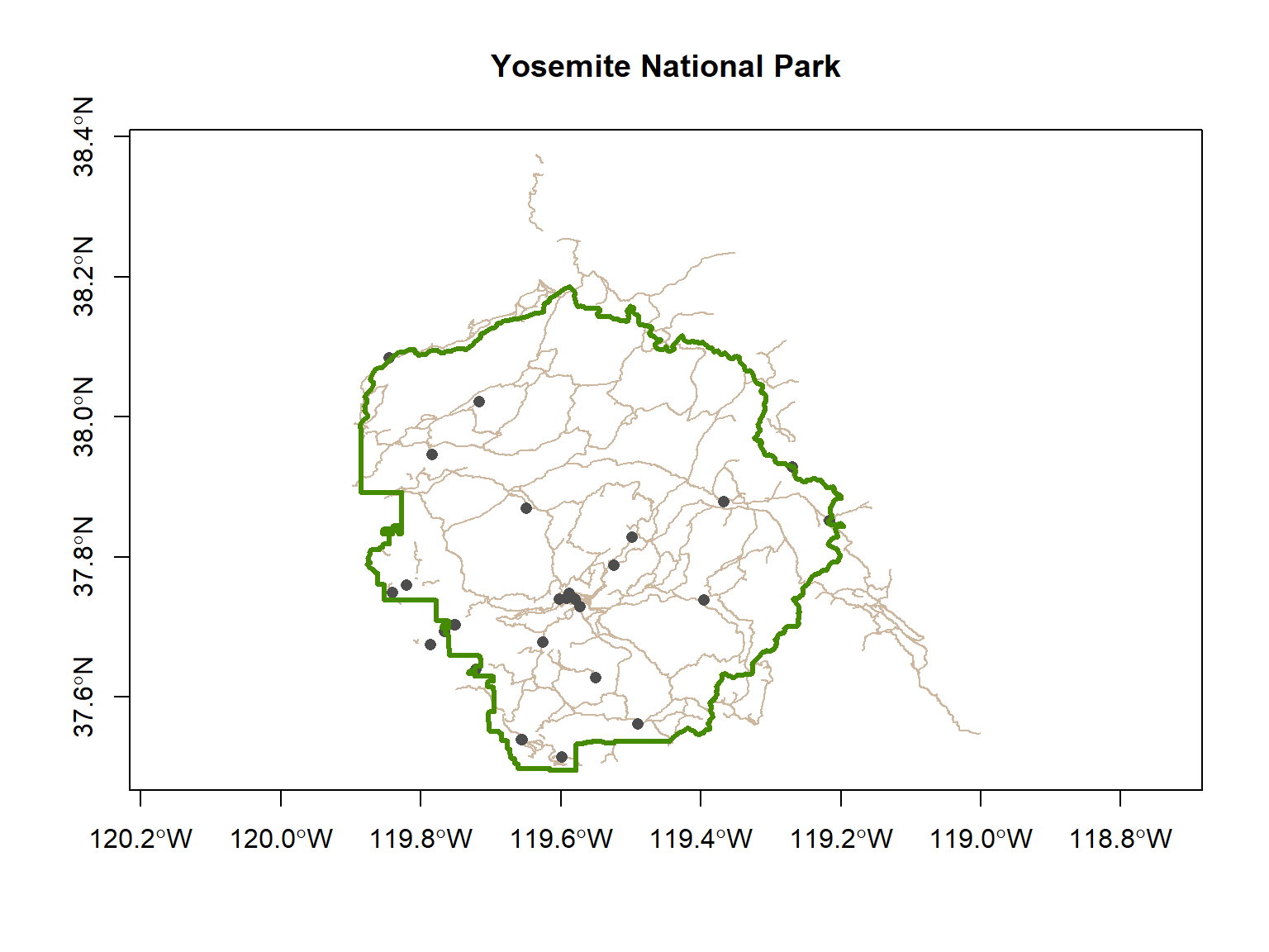
You can project one layer to match another without knowing the exact CRS. Just extract the CRS of the layer you’re trying to match with st_crs(), and use that as the second argument in st_transform().
Import the Yosemite roads and add those to your map. You may use the code below to get started.
[Solution]
## (Un)project the roads layer to geographic coordinates
yose_roads_ll <- st_transform(yose_roads_utm, 4269)
## Plot all four layers
plot(yose_trails_ll |> st_geometry(), asp=1, col="bisque3", axes=T, main="Yosemite")
plot(yose_roads_ll |> st_geometry(), col="navyblue", lwd=1, lty=5, add=TRUE)
plot(yose_hp_ll |> st_geometry(), col="gray30", pch=16, add=TRUE)
plot(yose_bnd_ll |> st_geometry(), col=NA, border="chartreuse4", lwd=3, add=TRUE)## [1] TRUE

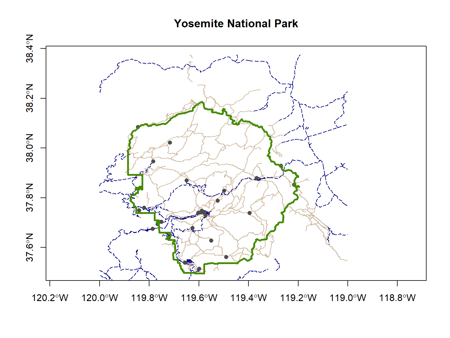
To turn a data frame into a sf object, use
st_as_sf(df, coords, crs)
where:
quakes is a dataframe that comes with R (in the datasets
package). Here we turn it into a sf data frame.
## Make a sf object from the built-in 'quakes' dataset
head(quakes)
quakes_sf <- st_as_sf(quakes, coords=c("long", "lat"), crs=4326)
plot(quakes_sf %>% st_geometry(), axes = TRUE, asp = 1)## lat long depth mag stations
## 1 -20.42 181.62 562 4.8 41
## 2 -20.62 181.03 650 4.2 15
## 3 -26.00 184.10 42 5.4 43
## 4 -17.97 181.66 626 4.1 19
## 5 -20.42 181.96 649 4.0 11
## 6 -19.68 184.31 195 4.0 12

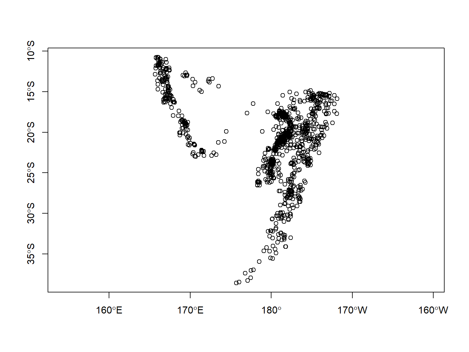
If you don’t know the datum for geographic coordinates, use WGS84 (epsg 4326).
You can export sf objects as Shapefiles and other formats using st_write()
If you name the output file with a standard extension (e.g., .shp, .kml), st_write() will know which format to use. Otherwise you have to add the driver argument.
By default, st_write() will throw an error if the output file already exists. To overwrite existing data (not recommended), add delete_dsn = TRUE.
| Function | Fix |
|---|---|
| tidyr::drop_na(geometry) | drop rows where there geometry column contains NA |
| sf::st_zm() | Drop Z and/or M dimensions from feature geometries |
| sf::st_is_valid() | check if features have geometry problems |
| sf::st_make_valid() | repair common geometry problems |
sf is relatively new, and many R packages still use the older data classes from the sp package.
Fortunately it’s relatively easy to convert back and forth:
## Please note that 'maptools' will be retired during October 2023,
## plan transition at your earliest convenience (see
## https://r-spatial.org/r/2023/05/15/evolution4.html and earlier blogs
## for guidance);some functionality will be moved to 'sp'.
## Checking rgeos availability: TRUE
data(wrld_simpl)
class(wrld_simpl)
## Convert sp to sf
wrld_simpl_sf <- sf::st_as_sf(wrld_simpl)
class(wrld_simpl_sf)
## Plot the sf object
plot(wrld_simpl_sf["REGION"])## [1] "SpatialPolygonsDataFrame"
## attr(,"package")
## [1] "sp"
## [1] "sf" "data.frame"
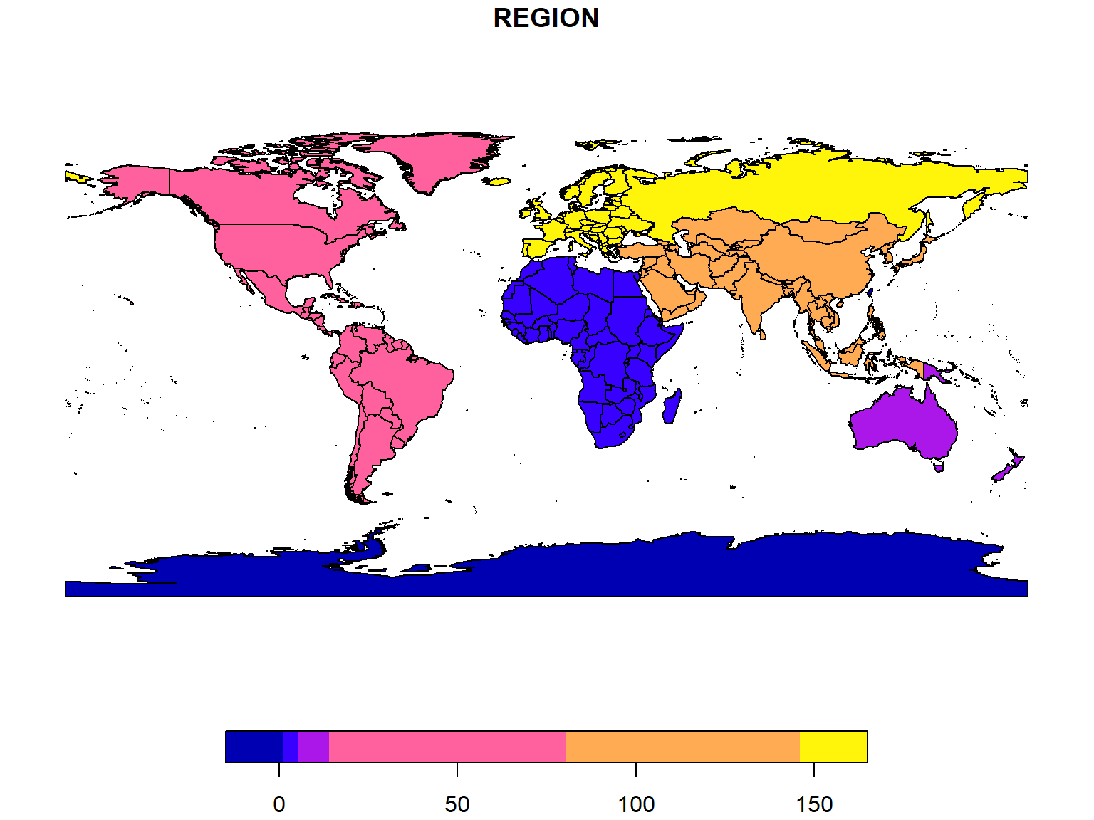
See also:
Today we saw how to:
st_as_Sf()Additional Resources
Geocomputation with R. Chapter 6: Reprojecting geographic data, Robin Lovelace
Geocomputation with R. Chapter 7 Geographic data I/O, Robin Lovelace