R for GIS
BayGeo, Spring 2024

Importing and Plotting Vector Data

`sf` Package

sf is a relatively new package for working with vector data. It combines the functionality of the older sp package, as well as select functionality from rgdal and rgeos.

library(sf)

sf stands for ‘simple feature’, which is a standard (developed by the Open Geospatial Consortium) for storing various geometry types in a hierarchical data model.

A ‘feature’ is just a representation of a thing in the real world (e.g. a building, a city…).

Package features:

uses established open source libraries: GDAL, GEOS, PROJ
fast IO (Input and Output)
enhanced plotting
objects are supported by an increasing number of other geospatial packages
alignment with other software that uses the simple features data model (e.g. QGIS, PostGIS)

`sf` functions

consistent function names (most start with st_)
|> pipe friendly!
everything you can do with a regular data frame, you can do with a sf data frame (almost)
integrated with the tidyverse packages

Importing Vector Data

To import spatial data, you have to specify a source and layer.

The Source can be a:

folder: "./gis_data"

geodatabase (which is really a folder): "./gis_data/yose_roads.gdb"

file: "trail_heads.kml", "cell_towers.geojson"

database connection string: "PG:dbname=postgis"

In sf functions, the argument where you provide the source is often named dsn (data source name)

The Layer can be a:

Shapefile name (minus the shp extension)

a named layer in the database / file

Import Functions

The two main functions for importing vector data are:

st_layers(source) - returns the names of available layers in a source

st_read(source, layer) - import into R

Most of the functions in the sf package start with st_, which stands for ‘space time’, and matches the names of similar functions in PostGIS.

To view the metadata of a layer before bringing it into R, use rgdal::ogrInfo()

Spatial Data File Formats

Shapefiles

Old format dating back to the early 90s
Originally from ESRI
Well-supported by nearly all GIS software
Actually requires 4-9 files with extensions *.shp, *.shx, *.prj, *.dbf, etc.
Column names in attribute table limited to 10 characters
Better options available today
st_read():

source - shp filename
layer - can be omitted

Example:

yose_bnd_ll <- st_read(dsn="./data", layer="yose_boundary")
yose_bnd_ll

## Reading layer `yose_boundary' from data source `D:\Workshops\R-Spatial\rspatial_mod\outputs\rspatial_bgs24\exercises\data' using driver `ESRI Shapefile'
## Simple feature collection with 1 feature and 11 fields
## Geometry type: POLYGON
## Dimension:     XY
## Bounding box:  xmin: -119.8864 ymin: 37.4947 xmax: -119.1964 ymax: 38.18515
## Geodetic CRS:  North_American_Datum_1983
## Simple feature collection with 1 feature and 11 fields
## Geometry type: POLYGON
## Dimension:     XY
## Bounding box:  xmin: -119.8864 ymin: 37.4947 xmax: -119.1964 ymax: 38.18515
## Geodetic CRS:  North_American_Datum_1983
##   UNIT_CODE                                                                           GIS_NOTES              UNIT_NAME  DATE_EDIT STATE REGION GNIS_ID
## 1      YOSE Lands - http://landsnet.nps.gov/tractsnet/documents/YOSE/METADATA/yose_metadata.xml Yosemite National Park 2016-01-27    CA     PW  255923
##       UNIT_TYPE CREATED_BY                                               METADATA PARKNAME                       geometry
## 1 National Park      Lands http://nrdata.nps.gov/programs/Lands/YOSE_METADATA.xml Yosemite POLYGON ((-119.8456 37.8327...

KML & KMZ

made popular with Google Earth
data and symbology are stored in one file
kmz files are simply zipped kml files
kml & kmz files can have more than one layer
limitations:

kmls support geographic coordinates only
you can not import a kmz file with st_read() (at least not on Windows). Unzip it first then import the doc.kml file
st_read() can not currently import the attribute table from a kml file on Windows (more info)
☞ Stay away from kml/kmz files if possible!

st_read():

source - kml filename
layer - name of a layer (required)

GeoJSON

GeoJSON is a good alternative to the Shapefile and KML formats
Supports all major geometry types, projections, attribute fields, etc.
GeoJSON typically stores one vector layer in one file that ends in .geojson (thus not very compact)
Format is plain text; can open and read in a text editor
st_read():

source - geojson filename
layer - named layer (optional if only 1 layer exists)

File Geodatabase

Proprietary spatial database format from ESRI
On disk is a folder with a .gdb extension
Supports all major feature types, projections, attribute tables, etc.
You can import (but not write to) a file geodatabase using the sf package
You can write to a geodatabase with the R-ArcGIS Bridge, if you have licensed copy of ArcGIS installed.
st_read():

source - folder containing the geodatabase
layer - named layer (required)

GeoPackage

GeoPackage is a relatively new open format for geospatial data. It is similar to a file geodatabase in that:

it can contain many layers
supports both raster and vector data
under the hood data are stored in a spatial database

The GeoPackage is different from a file geodatabase in that GeoPackages are:

a single file disk with a .gpkg extension (as opposed to a directory)
completely open source following a OGC standard
based on SQLite instead of a proprietary database format
cross-platform

st_read():

source - .gpkg filename
layer - named layer (required)

Spatial Databases

PostGIS - see rpostgis

SpatiaLite - see RSQLite.spatialite

The workshop datasets descriptions includes sample import code for most of the layers.

Basic Plotting sf Objects

To plot just the geometry of a sf object (i.e., no symbology from the attribute table), use st_geometry():

yose_bnd_ll <- st_read(dsn="./data", layer="yose_boundary", quiet=TRUE)

## Plot the geometry (outline) of the Yosemite boundary
plot(yose_bnd_ll |> st_geometry(), asp=1)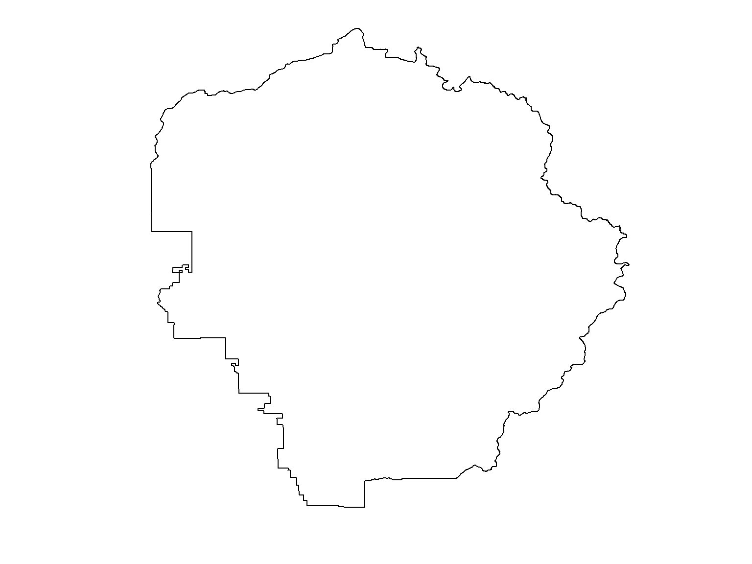

We add |> st_geometry() to indicate we want to plot the polygon with a single color/fill (more on that later).

The asp=1 argument sets the aspect ratio. It is optional but generally a good idea for spatial data.

Overlaying Layers

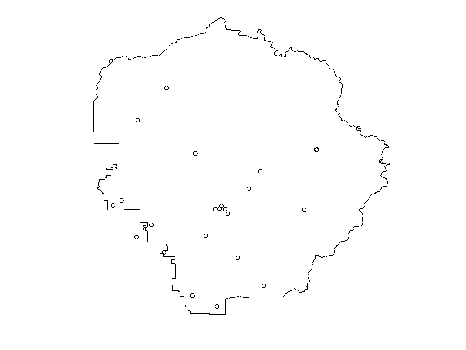
To overlay more than one layer on a plot:

both layers must have the same CRS (plot() does not reproject on the fly)
include add=TRUE to the second (and all subsequent) plot() statements

## Import the 'yosem_historic_places' layer 
yose_hp_ll <- st_read("./data/yose_historic_pts.kml", layer="yose_historic_places", quiet=TRUE)

## Plot the boundary
plot(yose_bnd_ll |> st_geometry(), asp=1)

## Add historic places
plot(yose_hp_ll |> st_geometry(), add=TRUE)

R Notebooks

R Notebooks are written in “R Markdown”, which combines text and R code.

R Notebook Exercise

nb_import-vector.Rmd

Import vector spatial data from a variety of file formats

preview notebook | answer key

Summary

In this section we saw how to:

import from Shapefiles, KMLs, GeoJson files, geodatabases, and GeoPackages
- st_layers() views the layer names
- st_read() imports the layer
use plot() for basic plotting
use plot(..., add=TRUE) to overlay additional layers with the same CRS

Additional Resources

Importing spatial data with rgdal, by Zev Ross

Plotting Simple Features, sf package Vignette

R for GISBayGeo, Spring 2024

sf Package

sf functions

Importing Vector Data

Import Functions

Spatial Data File Formats

Shapefiles

Example:

KML & KMZ

GeoJSON

File Geodatabase

GeoPackage

Spatial Databases

Basic Plotting sf Objects

Overlaying Layers

R Notebooks

R Notebook Exercise

Summary

END!

R for GIS
BayGeo, Spring 2024

`sf` Package

`sf` functions